Example Notebook : Cox

This notebook demonstrates the bayesian Cox model using SurvivalAnalysis workflow .

import pandas as pd
import numpy as np
import matplotlib.pyplot as plt
import arviz as az
import pymc as pm
import sys
import os


project_root = os.path.abspath(os.path.join(os.getcwd(), "../../../.."))


if project_root not in sys.path:
    sys.path.append(project_root)


from PyBH.SurvivalAnalysis.SurvivalAnalysis import SurvivalAnalysis
from PyBH.SurvivalAnalysis.pymc_models import Cox

1. Load Data

We use the Mastectomy dataset from the HSAUR R package. It describes survival times of women with breast cancer, comparing those who received a mastectomy only vs. those who received mastectomy + radiotherapy.

url = "https://vincentarelbundock.github.io/Rdatasets/csv/HSAUR/mastectomy.csv"

df_raw = pd.read_csv(url, index_col=0)

# Verify the cleanup
print("Columns:", df_raw.columns.tolist())
print(df_raw.head())

Columns: ['time', 'event', 'metastized']
          time  event metastized
rownames                        
1           23   True         no
2           47   True         no
3           69   True         no
4           70  False         no
5          100  False         no

2. Define Cutpoints

The Bayesian Cox model uses a piecewise constant baseline hazard. We need to define the time intervals (cutpoints). A good strategy is to use percentiles of the observed event times to ensure enough data in each interval.

n_intervals = 5
observed_times = df_raw['time'].values
cutpoints = np.percentile(observed_times[df_raw['event'] == 1], 
                          np.linspace(0, 100, n_intervals + 1)[1:-1])

print(f"Cutpoints: {cutpoints}")

Cutpoints: [23. 35. 50. 71.]

3. Initialize Model and Workflow

We create an instance of our PyMC Cox model and pass it to the SurvivalAnalysis manager.

cox_model = Cox(cutpoints=cutpoints, priors={"beta_sigma": 1.0})

analysis = SurvivalAnalysis(
    model=cox_model,
    data=df_raw,
    time_col="time",
    event_col="event",
    draws=2000,  
    tune=1000,
    chains=2,
    target_accept=0.9
)

Initializing NUTS using jitter+adapt_diag...

   -> Mode: Bayesian (PyMC)

Sequential sampling (2 chains in 1 job)
NUTS: [beta, lambda0]

Sampling 2 chains for 1_000 tune and 2_000 draw iterations (2_000 + 4_000 draws total) took 3 seconds.
We recommend running at least 4 chains for robust computation of convergence diagnostics

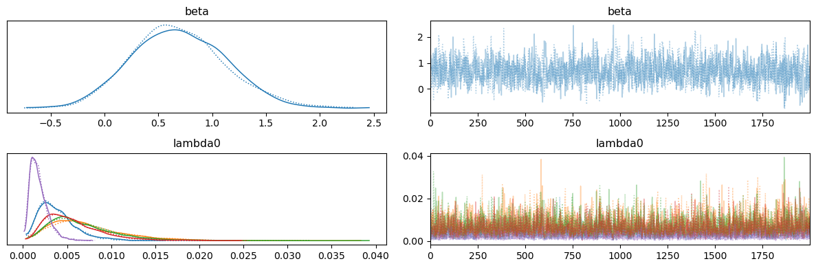
4. Diagnostics

The fit() method has already run (inside the constructor of SurvivalAnalysis). We can now check the Bayesian traces.

analysis.model.plot_traces()
print(analysis.model.print_summary())

                       mean     sd  hdi_3%  hdi_97%  mcse_mean  mcse_sd  \
beta[metastized_yes]  0.692  0.438  -0.092    1.528      0.013    0.008   
lambda0[Int_0]        0.004  0.002   0.001    0.008      0.000    0.000   
lambda0[Int_1]        0.007  0.004   0.001    0.015      0.000    0.000   
lambda0[Int_2]        0.007  0.004   0.001    0.014      0.000    0.000   
lambda0[Int_3]        0.006  0.003   0.001    0.011      0.000    0.000   
lambda0[Int_4]        0.002  0.001   0.000    0.004      0.000    0.000   

                      ess_bulk  ess_tail  r_hat  
beta[metastized_yes]    1166.0    1796.0    1.0  
lambda0[Int_0]          1718.0    2330.0    1.0  
lambda0[Int_1]          1890.0    2660.0    1.0  
lambda0[Int_2]          1728.0    2390.0    1.0  
lambda0[Int_3]          1777.0    2361.0    1.0  
lambda0[Int_4]          1823.0    2427.0    1.0  

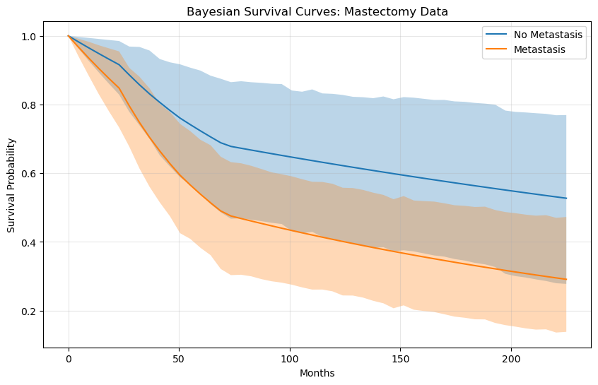
5. Survival Curves

Let’s plot the survival curves. Since SurvivalAnalysis.plot_survival_function currently plots a forest plot for coefficients, we can manually generate the survival curves using the predict_survival_function of our Cox class.

eval_times = np.linspace(0, df_raw.time.max(), 50)

# Create fake patients to compare: 
# Patient A: Metastasized = No (0)
# Patient B: Metastasized = Yes (1)
# Note: After one-hot encoding, check the column names in analysis.model._feature_names
print("Features used:", analysis.model._feature_names)

# Construct specific X matrix for prediction
# Assuming 'metastasized_yes' is the second column (index 1) after encoding
X_pred = np.array([
    [0], # Patient A (No metastasis)
    [1]  # Patient B (Metastasis)
])

surv_probs = analysis.model.predict_survival_function(eval_times, X_pred)

plt.figure(figsize=(10, 6))

# Plot Mean and 95% HDI for Patient A
mu_A = surv_probs[:, 0, :].mean(axis=0)
hdi_A = az.hdi(surv_probs[:, 0, :], hdi_prob=0.95)
plt.plot(eval_times, mu_A, label="No Metastasis")
plt.fill_between(eval_times, hdi_A[:,0], hdi_A[:,1], alpha=0.3)

# Plot Mean and 95% HDI for Patient B
mu_B = surv_probs[:, 1, :].mean(axis=0)
hdi_B = az.hdi(surv_probs[:, 1, :], hdi_prob=0.95)
plt.plot(eval_times, mu_B, label="Metastasis")
plt.fill_between(eval_times, hdi_B[:,0], hdi_B[:,1], alpha=0.3)

plt.title("Bayesian Survival Curves: Mastectomy Data")
plt.xlabel("Months")
plt.ylabel("Survival Probability")
plt.legend()
plt.grid(True, alpha=0.3)
plt.show()

Features used: ['metastized_yes']

/var/folders/sy/c1_rq0_x6dgdg_c_vymm1lnw0000gn/T/ipykernel_29870/2631143360.py:22: FutureWarning: hdi currently interprets 2d data as (draw, shape) but this will change in a future release to (chain, draw) for coherence with other functions
  hdi_A = az.hdi(surv_probs[:, 0, :], hdi_prob=0.95)
/var/folders/sy/c1_rq0_x6dgdg_c_vymm1lnw0000gn/T/ipykernel_29870/2631143360.py:28: FutureWarning: hdi currently interprets 2d data as (draw, shape) but this will change in a future release to (chain, draw) for coherence with other functions
  hdi_B = az.hdi(surv_probs[:, 1, :], hdi_prob=0.95)